Introduction
A lot of physical simulations can be converted into an optimization problem.
\[ \min_x f(x), \qquad f:\mathbb{R}^n \rightarrow \mathbb{R} \]where $x$ contains the variables, e.g., motion, material parameters, etc.
For simplicity, we consider no constraints and treat $f(x)$ as a general nonlinear function.
The general optimization is an iterative process, i.e.,
- Start from the current state: $x_n$
- Find a descent direction: $\Delta x_n$, such that $\nabla f(x_n)^T\Delta x_n<0$
- Calculate the next state: $x_{n+1}=x_n+\alpha\Delta x_n$, where $\alpha$ is a scaling factor
Check if $f(x_{n+1})<f(x_n)$. If not, reduce $\alpha$ and repeat the advancement step - Repeat steps ① ② ③ until the solution converges.
This tutorial focuses on step 2, i.e., finding a good moving direction for the current state. Specifically, we consider three commonly used optimizers: gradient descent, Newton method, and Broyden-Fletcher-Goldfarb-Shanno (BFGS).
Gradient descent
Let's start from the Taylor expansion at $x_n$
\[ f(x_n+\Delta x) = f(x_n)+\nabla f(x_n)^T\Delta x+O(\|\Delta x\|^2) \]$\nabla f(x_n)$ is the gradient of $f$ at $x_n$. Physically, under the Euclidean norm, it points to the direction with the maximum rate of increase of the function. Therefore, choosing $\Delta x=-\nabla f(x_n)$ gives the direction of steepest decrease.
For a unit moving direction $d$, the rate of change of $f$ is
\[ D_d f(x)=\nabla f(x)^T d. \]The maximum rate of increase is $|\nabla f(x)|$, obtained when $d$ points in the gradient direction. Thus, when using $\Delta x=-\nabla f(x_n)$, we need to choose $\alpha$ carefully. A small $\alpha$ makes the optimization extremely slow, though it is generally safe. On the contrary, a large $\alpha$ has the potential of overshooting, i.e., the advancement may bypass the true minimum and oscillate.
From the Taylor expansion, it's clear that gradient descent is a first-order method, as the higher-order term $O(|\Delta x|^2)$ is dropped.
Newton method
Newton method is a second-order method which can converge much faster than gradient descent. The key is that second-order information is incorporated into the advancement step.
Expand $f(x)$ at $x_n$ using the Taylor series as well.
\[ f(x_n+\Delta x) = f(x_n) + \nabla f(x_n)^T\Delta x + \frac{1}{2}\Delta x^T \nabla^2 f(x_n)\Delta x + O(\|\Delta x\|^3) \]The RHS is a quadratic approximation of $f(x)$. If the Hessian of this quadratic function is positive definite, the quadratic model has a unique global minimum. Denote the quadratic model as $m(\Delta x)$. The stationarity condition is
\[ \nabla_{\Delta x}m(\Delta x)=0. \]Take the derivative of the approximated quadratic function wrt $\Delta x$,
\[ \nabla_{\Delta x} \left( f(x_n)+\nabla f(x_n)^T\Delta x+\frac{1}{2}\Delta x^T \nabla^2 f(x_n)\Delta x \right)= \nabla f(x_n)+\nabla^2 f(x_n)\Delta x. \]Using the stationarity condition yields
\[ \nabla^2 f(x_n)\Delta x=-\nabla f(x_n). \]Denote $H=\nabla^2 f(x_n)$ and $g=\nabla f(x_n)$,
\[ H\Delta x=-g. \]Equivalently,
\[ \Delta x=-H^{-1}g. \]where $H$ is the Hessian matrix and $g$ is the gradient vector. In numerical implementation, we normally solve the linear system $H\Delta x=-g$ instead of explicitly calculating $H^{-1}$.
If $f(x)$ is itself a quadratic function with a positive-definite Hessian, a single Newton step finds the unique global minimum. For a general nonlinear function, more Newton steps are usually needed. But near a well-behaved minimum, Newton method can converge much faster than gradient descent.
Comparison between gradient descent and Newton method
The following figure clearly shows the difference. The function $f$ (red curve) is
\[ f(x)=x^3+8x^2+5x \]whose stationarity point is $x=-\frac{1}{3}$.
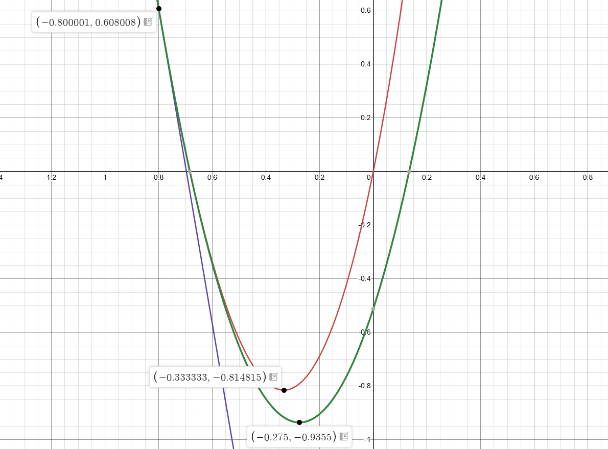
The initial guess is at $x_0=-0.8$. The blue and green curves are $f$'s 1st-order and 2nd-order polynomial fit at $x_0$, respectively. They correspond to gradient descent and Newton method's search direction. As shown in the figure, just one Newton iteration gives the next state $x_1=-0.375$ which is already fairly close to the true global minimum point.
One interesting thing about Newton method is that, close to a well-behaved minimum, a full Newton step with $\alpha=1$ is often accepted. However, line search is still generally needed when the current state is far from the minimum, even if the function is strictly convex.
If the Hessian is positive definite at the current state, i.e.,
\[ v^T H v>0,\qquad \forall v\in\mathbb{R}^N,\;v\neq0, \]then the Newton direction is a descent direction because
\[ g^T\Delta x=-g^T H^{-1}g<0. \]A positive-definite Hessian at every point is a sufficient condition for strict convexity, although it is not a necessary condition. If the Hessian is indefinite, Newton method may be attracted to a saddle point or point in a wrong direction. Therefore, practical Newton methods often use line search or trust-region methods to improve global convergence.
Another limitation of Newton method is that the computation and factorization of the Hessian can be computationally costly. When $N$ is small, the computation of $H$ is usually trivial. As $N$ increases, the computational and memory costs can become quite heavy. BFGS is one method targeted at this problem.
BFGS
BFGS avoids the computation of an exact Hessian by approximating it using gradient information from previous steps, i.e., $B\approx H$.
It's very intuitive to see how BFGS works from finite difference.
In 1D, $f'(x_n)$ and $f'(x_{n-1})$ are gradients of $f$. Then,
\[ f''(x_n) \approx \frac{f'(x_n)-f'(x_{n-1})}{x_n-x_{n-1}}. \]This approximation converges to the true second derivative when $x_n-x_{n-1}$ approaches zero, assuming the function is sufficiently smooth.
For the general ND case, define
\[ \begin{cases} s_n=x_n-x_{n-1}\\ y_n=\nabla f(x_n)-\nabla f(x_{n-1}). \end{cases} \]The change in gradient satisfies
\[ y_n = \int_0^1 \nabla^2 f(x_{n-1}+t s_n)s_n\,dt. \]If the Hessian does not change much along this step, we have
\[ Hs_n\approx y_n. \]Therefore, BFGS chooses an approximate Hessian $B_n$ such that
\[ B_n s_n=y_n, \]which is called the secant equation.
However, directly solving this equation cannot uniquely determine $B_n$, because it provides only $N$ scalar equations for the $N^2$ entries of a general $N\times N$ matrix. Therefore, there are infinitely many matrices satisfying the secant equation. BFGS chooses a symmetric matrix that satisfies the secant equation while making a controlled change from the previous approximation $B_{n-1}$. The update is the so-called rank-two correction,
\[ B_n = B_{n-1} - \frac{B_{n-1}s_n s_n^T B_{n-1}} {s_n^T B_{n-1}s_n} + \frac{y_n y_n^T} {y_n^T s_n} \qquad \cdots\cdots \text{(1)} \]It is called a rank-two correction because $B_n-B_{n-1}$ is the sum of two rank-one matrices. $B_n$ itself is normally a full-rank matrix.
This expression may look intimidating, but conceptually it does two things: 1) remove the old curvature information along $s_n$, i.e., the second term; 2) add the newly observed curvature information, i.e., the third term.
Multiplying $s_n$ on both sides of Eq.1 gives
\[ \begin{aligned} B_n s_n &= B_{n-1}s_n - B_{n-1}s_n \frac{s_n^T B_{n-1}s_n} {s_n^T B_{n-1}s_n} + y_n \frac{y_n^T s_n} {y_n^T s_n} \\ &= B_{n-1}s_n - B_{n-1}s_n + y_n \\ &= y_n. \end{aligned} \]Therefore, the second term removes the old prediction $B_{n-1}s_n$ of the gradient change along $s_n$. The third term adds the observed gradient change $y_n$, so that the new approximation satisfies the secant equation $B_n s_n=y_n$.
Another important condition in BFGS is the curvature condition
\[ y_n^T s_n>0. \]If $B_{n-1}$ is positive definite and $y_n^T s_n>0$, the BFGS update preserves the positive definiteness of $B_n$. Therefore,
\[ \Delta x_n=-B_n^{-1}g_n \]remains a descent direction. In practice, BFGS is often combined with a Wolfe line search, which helps satisfy this curvature condition.
Under suitable smoothness, convexity, and line-search conditions, BFGS can achieve superlinear local convergence. Gradient descent typically has linear convergence for smooth strongly convex problems, while Newton method can achieve quadratic local convergence near a well-behaved minimum. Therefore, BFGS is often viewed as a compromise between the low computational cost of gradient descent and the fast convergence of Newton method.