When I learned fluid dynamics as an undergraduate, the most difficult part for me to understand was the material derivative. I did not understand why something as simple as acceleration could yield such a complicated expression. Intuitively, acceleration is just the time derivative of velocity. Anyone with high-school calculus knowledge can write
\[ \mathbf{a}=\frac{d\mathbf{v}}{dt}. \]However, when velocity is represented as an Eulerian field $\mathbf{v}(\mathbf{x},t)$, writing
\[ \mathbf{a}=\frac{\partial \mathbf{v}}{\partial t} \]is only partially correct. The partial derivative measures the change of velocity at a fixed spatial location, whereas acceleration follows a moving material particle. The missing contribution is exactly what the material derivative accounts for.
Intuitive
The Lagrangian and Eulerian views are two different ways of describing motion. Consider a car racing along a road. If you sit at a fixed location beside the road, say at a bus station, you see the car move toward you and then disappear into the distance. This is an Eulerian view because you are fixed in space.
At the same time, imagine that your friend is sitting in the car. Your friend's view is Lagrangian because your friend moves with the object.
Now consider a temperature field $T$ in some region. If you want to know the temperature at any point and at any time, you need both the spatial position $\mathbf{x}$ and the time $t$. Thus, the temperature field can be written as
\[ T=T(\mathbf{x},t). \]The material derivative answers a specific question: how does this field change with time as observed by a material particle moving through the field?
Derivation
The material derivative is the time derivative taken while following a material particle. When a field is represented in Eulerian coordinates, the material derivative can be written as
\[ \frac{D}{Dt}:=\frac{\partial}{\partial t}+\mathbf{v}\cdot\nabla. \]Before going deeper into the derivation, we need to distinguish between material coordinates and spatial coordinates.
A material coordinate $\mathbf{X}$ labels a particular material particle in the reference configuration. The spatial coordinate $\mathbf{x}$ gives the current position of that particle in physical space. The motion is
\[ \mathbf{x}=\boldsymbol{\phi}(\mathbf{X},t). \]If the map is invertible, we can also write
\[ \mathbf{X}=\boldsymbol{\phi}^{-1}(\mathbf{x},t). \]Now suppose a scalar Eulerian field $f(x,t)$ is defined in 1D. A material particle labeled by $X$ moves along the trajectory
\[ x=\phi(X,t). \]The value of the field observed by that particle is therefore
\[ \hat{f}(X,t)=f\!\left(\phi(X,t),t\right). \]We want to know how the observed value changes with time while keeping the material particle $X$ fixed:
\[ \frac{D f}{Dt} := \left.\frac{\partial \hat{f}(X,t)}{\partial t}\right|_X. \]According to the chain rule,
\[ \begin{aligned} \frac{D f}{Dt} &= \frac{\partial f}{\partial t} + \frac{\partial f}{\partial x} \frac{\partial \phi(X,t)}{\partial t}. \end{aligned} \]The velocity of that material particle is
\[ v(x,t)=\left.\frac{\partial \phi(X,t)}{\partial t}\right|_X. \]Therefore, in 1D,
\[ \boxed{ \frac{D f}{Dt} = \frac{\partial f}{\partial t} + v\frac{\partial f}{\partial x} }. \]In 3D, the same chain rule gives
\[ \begin{aligned} \frac{D f}{Dt} &= \frac{\partial f}{\partial t} + v_x\frac{\partial f}{\partial x} + v_y\frac{\partial f}{\partial y} + v_z\frac{\partial f}{\partial z} \\ &= \frac{\partial f}{\partial t} + \begin{bmatrix} v_x & v_y & v_z \end{bmatrix} \begin{bmatrix} \dfrac{\partial f}{\partial x}\\[4pt] \dfrac{\partial f}{\partial y}\\[4pt] \dfrac{\partial f}{\partial z} \end{bmatrix} \\ &= \frac{\partial f}{\partial t} + \mathbf{v}\cdot\nabla f. \end{aligned} \]Here, $\nabla$ is the nabla operator or del operator. When it acts on a scalar field, it is the gradient operator:
\[ \nabla f = \begin{bmatrix} \dfrac{\partial f}{\partial x}\\[4pt] \dfrac{\partial f}{\partial y}\\[4pt] \dfrac{\partial f}{\partial z} \end{bmatrix}. \]Thus,
\[ \boxed{ \frac{D f}{Dt} = \frac{\partial f}{\partial t} + \mathbf{v}\cdot\nabla f }. \]Now look at the expression on the RHS. The first term measures the filed's internal change in time, which is irrelevent to the particle's motion. The second term measures the change due to particle's movement in the field. $\mathbf{v}$ is the particle's velocity at time $t$ and $x$. $\nabla f$ is the field's value difference per unit change. Their dot product $\mathbf{v}.\nabla f$ is precisely the field value change due to particle movement.
\[ \boxed{ \text{change seen by a moving particle} = \text{change at a fixed spatial point} + \text{change due to motion through the field} }. \]The intuitive way to understand the material derivative is to view it as an ordinary chain rule applied along a particle trajectory. Suppose
\[ f=f(a,b), \qquad a=a(b). \]Then
\[ \frac{df}{db} = \frac{\partial f}{\partial b} + \frac{\partial f}{\partial a} \frac{da}{db}. \]The material derivative is exactly the same idea. Here,
\[ f=f(\mathbf{x},t), \qquad \mathbf{x}=\mathbf{x}_p(t), \]where $\mathbf{x}_p(t)$ is the trajectory of a material particle. Therefore,
\[ \frac{d}{dt}f(\mathbf{x}_p(t),t) = \frac{\partial f}{\partial t} + \nabla f\cdot\frac{d\mathbf{x}_p}{dt}. \]Since
\[ \frac{d\mathbf{x}_p}{dt}=\mathbf{v}, \]we obtain the material derivative.
Because this relation holds for any sufficiently smooth scalar field $f$, we can write the material derivative operator itself as
\[ \boxed{ \frac{D}{Dt} = \frac{\partial}{\partial t} + \mathbf{v}\cdot\nabla }. \]For the Eulerian velocity field itself, $\mathbf{v}(\mathbf{x},t)$, the acceleration of a material particle is
\[ \boxed{ \mathbf{a} = \frac{D\mathbf{v}}{Dt} = \frac{\partial\mathbf{v}}{\partial t} + (\mathbf{v}\cdot\nabla)\mathbf{v} }. \]This explains why $\partial\mathbf{v}/\partial t$ alone is generally not the acceleration in an Eulerian description.
Lagrangian view
The material derivative itself is not exclusively Eulerian or Lagrangian. It always means the rate of change observed while following a material particle. What changes is its mathematical representation.
In an Eulerian description, a field is written as
\[ f=f(\mathbf{x},t), \]and the material derivative is
\[ \frac{D f}{Dt} = \frac{\partial f}{\partial t} + \mathbf{v}\cdot\nabla f. \]In a Lagrangian description, we instead write the same physical field as
\[ \hat{f}(\mathbf{X},t) = f(\boldsymbol{\phi}(\mathbf{X},t),t). \]Because the material coordinate $\mathbf{X}$ follows the particle, the material derivative becomes simply
\[ \boxed{ \frac{D f}{Dt} = \left.\frac{\partial \hat{f}}{\partial t}\right|_{\mathbf{X}} }. \]This is why standard solid FEM, which usually uses a Lagrangian description in which the mesh follows the material, does not contain an explicit convective term.
Material derivative of the spatial coordinate
Now consider the Eulerian identity field
\[ \mathbf{g}(\mathbf{x},t)=\mathbf{x}. \]At a fixed spatial location $\mathbf{x}$, this field has no explicit time dependence, so
\[ \left.\frac{\partial \mathbf{g}}{\partial t}\right|_{\mathbf{x}}=\mathbf{0}. \]However, its material derivative is not zero. Applying the material derivative componentwise,
\[ \begin{aligned} \frac{D\mathbf{g}}{Dt} &= \frac{\partial\mathbf{g}}{\partial t} + (\mathbf{v}\cdot\nabla)\mathbf{g} \\ &= \mathbf{0} + \begin{bmatrix} \mathbf{v}\cdot\nabla x \\ \mathbf{v}\cdot\nabla y \\ \mathbf{v}\cdot\nabla z \end{bmatrix} \\ &= \begin{bmatrix} v_x \\ v_y \\ v_z \end{bmatrix} \\ &= \mathbf{v}. \end{aligned} \]Therefore,
\[ \boxed{ \frac{D\mathbf{x}}{Dt}=\mathbf{v} }. \]There is no contradiction between
\[ \left.\frac{\partial\mathbf{x}}{\partial t}\right|_{\mathbf{x}}=\mathbf{0} \]and
\[ \frac{D\mathbf{x}}{Dt}=\mathbf{v}. \]The first derivative is taken at a fixed spatial coordinate, while the second derivative follows a moving material particle.
A concrete example
Here we give a concrete example using finite difference.
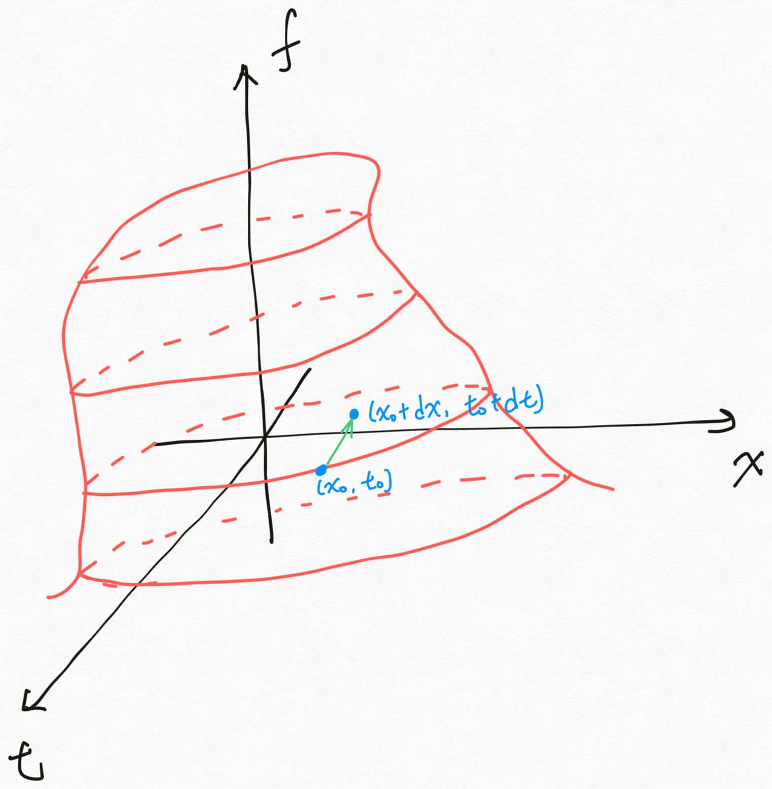
In the above figure, the field varies with both time $t$ and space $x$. A particle moves from the current the state $(x_{0},t_{0})$ to the next state $(x_{0} + dx, t_{0}+dt)$ for a tiny period of time $dt$.
According to the definition of material derivative:
\[ \frac{Df}{Dt} = \lim_{dt\to 0} \frac{ f(x_0+dx,t_0+dt)-f(x_0,t_0) }{ dt }. \tag{1} \]Because we are following a particle's trajectory, $dx$ is not an independent variable. For a tiny time change $dt$, the displacement is
\[ dx=v\,dt. \]Therefore, Eq. (1) becomes
\[ \frac{Df}{Dt} = \lim_{dt\to 0} \frac{ f(x_0+v\,dt,t_0+dt)-f(x_0,t_0) }{ dt }. \tag{2} \]Taylor expansion in time
Rewrite the first term in the numerator using a Taylor expansion around $t_0$:
\[ f(x_0+v\,dt,t_0+dt) = f(x_0+v\,dt,t_0) + f_t(x_0+v\,dt,t_0)\,dt + O(dt^2). \]Thus,
\[ f(x_0+v\,dt,t_0+dt) \approx f(x_0+v\,dt,t_0) + f_t(x_0+v\,dt,t_0)\,dt. \]Further Taylor expansion in space
For the first term,
\[ f(x_0+v\,dt,t_0) = f(x_0,t_0) + f_x(x_0,t_0)\,v\,dt + O(dt^2). \]For the time derivative term,
\[ f_t(x_0+v\,dt,t_0) = f_t(x_0,t_0) + f_{tx}(x_0,t_0)\,v\,dt + O(dt^2). \]Multiplying this second expansion by $dt$ gives
\[ f_t(x_0+v\,dt,t_0)\,dt = f_t(x_0,t_0)\,dt + f_{tx}(x_0,t_0)\,v\,dt^2 + O(dt^3). \]Hence, keeping only first-order terms,
\[ f(x_0+v\,dt,t_0+dt) \approx f(x_0,t_0) + f_x(x_0,t_0)\,v\,dt + f_t(x_0,t_0)\,dt. \]Substitute into the definition
Substituting into Eq. (2),
\[ \frac{Df}{Dt} = \lim_{dt\to 0} \frac{ f(x_0,t_0) + f_x(x_0,t_0)\,v\,dt + f_t(x_0,t_0)\,dt - f(x_0,t_0) }{ dt }. \]The $f(x_0,t_0)$ terms cancel:
\[ \frac{Df}{Dt} = \lim_{dt\to 0} \left[ f_t(x_0,t_0) + v\,f_x(x_0,t_0) \right]. \]Therefore,
\[ \boxed{ \frac{Df}{Dt} = f_t(x_0,t_0) + v\,f_x(x_0,t_0) } \]or equivalently,
\[ \boxed{ \frac{Df}{Dt} = \frac{\partial f}{\partial t} + v\frac{\partial f}{\partial x} }. \]For a multidimensional field,
\[ \boxed{ \frac{Df}{Dt} = \frac{\partial f}{\partial t} + \mathbf{v}\cdot\nabla f }. \]