This is Part II of the differentiable simulation tutorial series. Part I is about quasi-static FEM simulation(here). This tutorial entends it to dynamic simulation
(1) Problem statement
We use the same free-hanging 3D beam and three optimizable material parameters as in the static case. The same vertex is tracked. But instead of trying to match the tracked vertex position with the target position at the final equilibrium configuration, we want the tracked vertex to follow a reference trajectory defined at each timestep. Therefore, the total loss of the system is defined as:
\[ \begin{aligned} L &= \sum_{n=0}^{N} L^n \\ &= \sum_{n=0}^{N} \frac{1}{2s^2}\left\|x^n_{\mathrm{tracked}}(q^n) - x^n_{\mathrm{target}}\right\|^2 \end{aligned} \tag{1} \]where $x^n_{\mathrm{tracked}}(q^n)$ and $x^n_{\mathrm{target}}$ are the tracked-point position and target-point position at the $n$th timestep, respectively.
Consider an implicit Euler FEM simulation. The time-step incremental potential from timestep $n$ to $n+1$ is:
\[ \begin{aligned} Φ^n(q^{n+1},q^{n},v^{n},θ) &= E^n_{inertia}+\Pi(q^{n+1},\theta)\\ &= \frac{1}{2h^2} (q^{n+1}-q^n-hv^n)^T M(\rho) (q^{n+1}-q^n-hv^n) \\ &\qquad+ \sum_e E_e(q^{n+1},E,\nu) + E_g(q^{n+1},\rho). \end{aligned} \tag{2} \]where $q^{n}$ and $q^{n+1}$ are the vertex positions at timesteps $n$ and $n+1$, respectively. $v^n$ is the velocity at timestep $n$, $h$ is the timestep size, and $M(\rho)$ is the lumped mass matrix. $E^n_{inertia}= \frac{1}{2h^2} (q^{n+1}-q^n-hv^n)^T M(\rho) (q^{n+1}-q^n-hv^n)$ is the incremental inertial term. $\Pi(q^{n+1},\theta)$ is the potential energy evaluated at the next step.
Note that this incremental potential is different from the total mechanical energy:
\[ \begin{aligned} E^{n+1}(q^{n+1},v^{n+1},θ) &=T^{n+1}(v^{n+1},θ)+Π(q^{n+1},θ) \\ &=\frac{1}{2}(v^{n+1})^TM(\rho)v^{n+1}+\sum_e E_e(q^{n+1},E,\nu) + E_g(q^{n+1},\rho) \end{aligned} \tag{3} \]The former is an incremental potential associated with the transition from timestep $n$ to $n+1$. Its stationarity condition gives the dynamic equilibrium equation, i.e.,
\[ R^n(q^{n+1},q^{n},v^{n},\theta)=\frac{\partial \Phi^n}{\partial q^{n+1}} \tag{4} \]Therefore, at each timestep $n=0,\ldots,N-1$, we solve the implicit equation $R^{n}$.
\[ R^{n}(q^{n+1}, q^n, v^n, \theta) = 0 \tag{5} \]For a simulation with states $n=0,\ldots,N$, the residual $R^n$ is defined for $n=0,\ldots,N-1$, because each residual advances the state from timestep $n$ to $n+1$.
The updated configuration $q^{n+1}$ can be obtained accordingly.
The next step's velocity $v^{n+1}$ can be easily computed after $q^{n+1}$ is known.
\[ v^{n+1} = \frac{q^{n+1}-q^n}{h} \tag{6} \]Differentiate Eq. 5:
\[ dR^{n} = \frac{\partial R^{n}}{\partial q^{n+1}}\,dq^{n+1} + \frac{\partial R^{n}}{\partial q^n}\,dq^n + \frac{\partial R^{n}}{\partial v^n}\,dv^n + \frac{\partial R^{n}}{\partial \theta}\,d\theta \tag{7} \]Assuming the solution converges at the end of each timestep, $R^{n}=0$ holds. As a result, $dR^{n}=0$ holds as well.
Denote:
\[ R_{q^{n+1}} = \frac{\partial R^{n}}{\partial q^{n+1}}, \qquad R_{q^{n}} = \frac{\partial R^{n}}{\partial q^n}, \qquad R_{v_{n}} = \frac{\partial R^{n}}{\partial v^n}, \qquad R_{\theta} = \frac{\partial R^{n}}{\partial \theta} \tag{8} \]These derivatives can be computed using automatic differentiation frameworks as well.
Substituting Eq. 8 into Eq. 7 yields:
\[ R_{q^{n+1}}\,dq^{n+1} + R_{q^{n}}\,dq^n + R_{v_{n}}\,dv^n + R_{\theta}\,d\theta = 0 \tag{9} \](2) Direct method
Divide Eq. 9 by $d\theta$ on both sides:
\[ R_{q^{n+1}}\frac{dq^{n+1}}{d\theta} + R_{q^{n}}\frac{dq^n}{d\theta} + R_{v_{n}}\frac{dv^n}{d\theta} + R_{\theta} = 0 \tag{10} \]Define
\[ Q^{n+1}_{\theta} = \frac{dq^{n+1}}{d\theta}, \qquad Q^{n}_{\theta} = \frac{dq^n}{d\theta}, \qquad V^{n}_{\theta} = \frac{dv^n}{d\theta} \tag{11} \]Substituting Eq. 11 into Eq. 10 yields:
\[ R_{q^{n+1}}Q^{n+1}_{\theta} + R_{q^{n}}Q^{n}_{\theta} + R_{v_{n}}V^{n}_{\theta} + R_{\theta} = 0 \]Assuming $R_{q^{n+1}}$ is invertible,
\[ Q^{n+1}_{\theta} = -\left(R_{q^{n+1}}\right)^{-1}\left(R_{q^{n}}Q^{n}_{\theta} + R_{v_{n}}V^{n}_{\theta} + R_{\theta}\right) \tag{12} \]Eq. 6 relates $q^{n+1}$ and $q^n$ with $v^{n+1}$. Differentiate both sides:
\[ dv^{n+1} = \frac{1}{h}\left(dq^{n+1}-dq^n\right) \tag{13} \]Divide by $d\theta$ on both sides:
\[ \frac{dv^{n+1}}{d\theta} = \frac{1}{h}\left( \frac{dq^{n+1}}{d\theta} - \frac{dq^n}{d\theta} \right) \] \[ \Rightarrow\quad V^{n+1}_{\theta}= \frac{1}{h}\left(Q^{n+1}_{\theta}-Q^{n}_{\theta}\right) \tag{14} \]Combine Eq. 12 and Eq. 14:
\[ \begin{cases} Q^{n+1}_{\theta} = -\left(R_{q^{n+1}}\right)^{-1}\left(R_{q^{n}}Q^{n}_{\theta} + R_{v_{n}}V^{n}_{\theta} + R_{\theta}\right),\\[6pt] V^{n+1}_{\theta} = \dfrac{1}{h}\left(Q^{n+1}_{\theta}-Q^{n}_{\theta}\right). \end{cases} \tag{15} \]Given the initial values at the beginning of the simulation:
\[ Q^0_{\theta} = 0, \qquad V^0_{\theta} = 0 \tag{16} \]because the initial position and velocity are independent of the material parameters. Therefore, $Q^{n}_{\theta}=\frac{dq^{n}}{d\theta}$ can be calculated recursively at each timestep.
The derivative of the total loss with respect to the material parameters $\theta$ is:
\[ \begin{aligned} \frac{dL}{d\theta} &= \sum_{n=0}^{N}\frac{dL^n}{d\theta} \\ &= \sum_{n=0}^{N}\left(\frac{dq^n}{d\theta}\right)^T\frac{dL^n}{dq^n} \\ &= \sum_{n=0}^{N} {(Q^{n}_{\theta})}^TL^n_{q} \end{aligned} \tag{17} \](3) Adjoint method
Define $J^n$ as the remaining loss from timestep $n$ onward, including the loss at timestep $n$. For $n=0,\ldots,N-1$:
\[ J^n(q^n, v^n; \theta) = L^n + J^{n+1}(q^{n+1}, v^{n+1}; \theta) \tag{18} \]Or equivalently,
\[ J^n(q^n, v^n; \theta) = \sum_{m=n}^{N} L^m \tag{19} \]where “;” separates the state variables (qn,vn)(q^n,v^n) from the model parameters $\theta$. The same $\theta$ is used throughout a forward simulation. Note $J^n$ depends on both $q^{n}$ and $v^n$ for two reasons. First, the current position directly contributes to the current timestep's loss. Second, the current state determines future states and influences the total loss implicitly.
Differentiate both sides of Eq. 18.
On the LHS:
\[ dJ^n = \left(\frac{\partial J^n}{\partial q^n}\right)^T\!dq^n + \left(\frac{\partial J^n}{\partial v^n}\right)^T\!dv^n + \left(\frac{\partial J^n}{\partial \theta}\right)^T\!d\theta \tag{20} \]On the RHS:
\[ \begin{aligned} dJ^{n+1} + dL^n ={}& \left(\frac{\partial J^{n+1}}{\partial q^{n+1}}\right)^T\!dq^{n+1} + \left(\frac{\partial J^{n+1}}{\partial v^{n+1}}\right)^T\!dv^{n+1} \\ &+ \left(\frac{\partial J^{n+1}}{\partial \theta}\right)^T\!d\theta + \left(\frac{\partial L^n}{\partial q^n}\right)^T\!dq^n \end{aligned} \tag{21} \]Substituting Eq. 13 into Eq. 21 yields:
\[ \begin{aligned} dJ^{n+1} + dL^n ={}& \left(\frac{\partial J^{n+1}}{\partial q^{n+1}}\right)^T\!dq^{n+1} + \left(\frac{\partial J^{n+1}}{\partial v^{n+1}}\right)^T \frac{1}{h}\left(dq^{n+1}-dq^n\right) \\ &+ \left(\frac{\partial J^{n+1}}{\partial \theta}\right)^T\!d\theta + \left(\frac{\partial L^n}{\partial q^n}\right)^T\!dq^n \end{aligned} \tag{22} \]Define:
\[ {J}^n_q = \frac{\partial J^n}{\partial q^n}, \qquad {J}^{n}_v = \frac{\partial J^n}{\partial v^n}, \qquad {J}^{n}_{\theta} = \frac{\partial J^n}{\partial \theta} \]where ${J}^n_q$ and ${J}^n_v$ are state adjoints or costates, while ${J}^{n}_{\theta}$ is the accumulated sensitivity of the remaining loss with respect to the parameters..
They represent the sensitivity of the remaining loss with respect to the current state variables and parameters.
Eq. 20 becomes:
\[ dJ^n = ({J}^n_q)^T\,dq^n + ({J}^{n}_v)^T\,dv^n + ({J}^{n}_{\theta})^T\,d\theta \tag{23} \]Eq. 22 becomes:
\[ \begin{aligned} dJ^{n+1} + dL^n ={}& ({J}^{n+1}_q)^T\,dq^{n+1} + ({J}^{n+1}_v)^T\frac{1}{h}\left(dq^{n+1}-dq^n\right) + ({J}^{n+1}_{\theta})^T\,d\theta + \left(\frac{\partial L^n}{\partial q^n}\right)^T\!dq^n \\ ={}& \left({J}^{n+1}_q+\frac{{J}^{n+1}_v}{h}\right)^T dq^{n+1} + \left(\frac{\partial L^n}{\partial q^n}-\frac{{J}^{n+1}_v}{h}\right)^T dq^n + ({J}^{n+1}_{\theta})^T\,d\theta \end{aligned} \tag{24} \]Assuming $R_{q^{n+1}}$ is invertible, Eq. 9 states:
\[ dq^{n+1} = -\left(R_{q^{n+1}}\right)^{-1}\left(R_{q^{n}}\,dq^n + R_{v_{n}}\,dv^n + R_{\theta}\,d\theta\right) \tag{25} \]Substitute Eq. 25 into Eq. 24:
\[ \begin{aligned} dJ^{n+1}+dL^n ={}& -\gamma_n^T \left(R_{q^{n+1}}\right)^{-1} \left(R_{q^{n}}\,dq^n+R_{v_{n}}\,dv^n+R_{\theta}\,d\theta\right) \\ &+ \left(\frac{\partial L^n}{\partial q^n}-\frac{{J}^{n+1}_v}{h}\right)^T dq^n + ({J}^{n+1}_{\theta})^T d\theta \\ ={}& \left( \frac{\partial L^n}{\partial q^n} - \frac{{J}^{n+1}_v}{h} - R_{q^{n}}^T\left(R_{q^{n+1}}\right)^{-T}\gamma_n \right)^T dq^n \\ &- \left(R_{v_{n}}^T\left(R_{q^{n+1}}\right)^{-T}\gamma_n\right)^T dv^n + \left({J}^{n+1}_{\theta}- R_{\theta}^T\left(R_{q^{n+1}}\right)^{-T}\gamma_n\right)^T d\theta \\ ={}& \left( L^n_{q} - \frac{{J}^{n+1}_v}{h} - R_{q^{n}}^T\lambda_n \right)^T dq^n + \left(-R_{v^{n}}^T\lambda_n\right)^T dv^n \\ &+ \left({J}^{n+1}_{\theta}-R_{\theta}^T\lambda_n\right)^T d\theta \end{aligned} \tag{26} \]We denote
\[ \gamma_n = {J}^{n+1}_q + \frac{{J}^{n+1}_v}{h}, \qquad \left(R_{q^{n+1}}\right)^T\lambda_n = \gamma_n, \qquad L^n_{q} = \frac{\partial L^n}{\partial q^n} \]where $\lambda_{n}$ is the adjoint variable which measures the sensitivity of future loss wrt the timestep $n$ residual equation variation (up to the residual sign convention). $\gamma_n$ is the future loss sensitivity wrt the state variable $q^{n+1}$ accounting for the contribution of velocity. This is the dynamic counterpart of the static adjoint equation, $R_q^T\lambda = L_q$, in our Part-I tutorial.
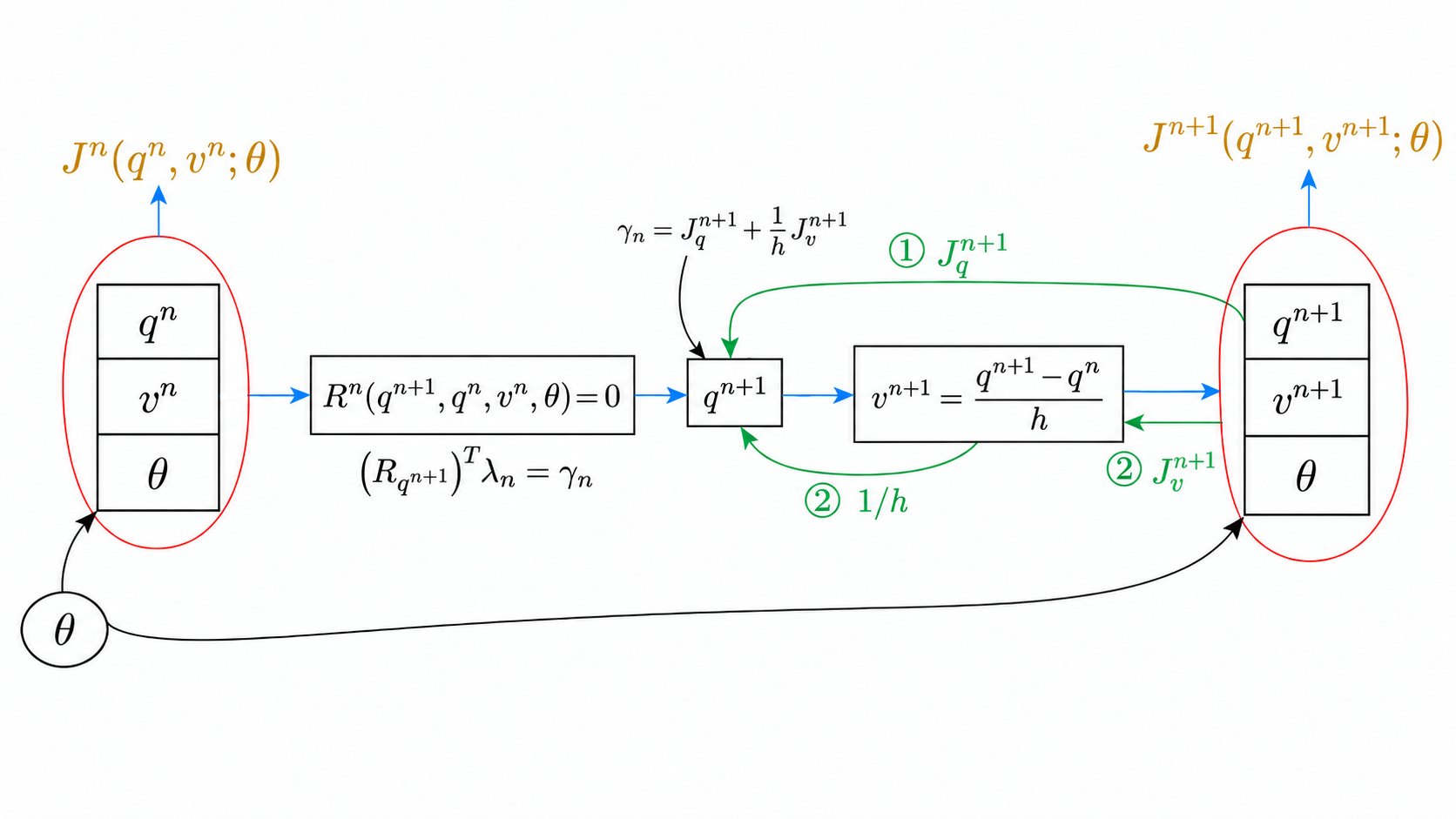 Compare Eq. 23 and Eq. 26:
Since $J^N=L^N$ and $L^N$ depends only on $q^N$, the terminal conditions are
\[ J_q^N = L_q^N, \qquad J_v^N = 0, \qquad J_\theta^N = 0. \]The adjoint recursion is then evaluated backward for $n=N-1,\ldots,0$. Because the initial position and velocity are independent of $\theta$, the final gradient is
\[ \frac{dL}{d\theta}=J_\theta^0. \](4) Conclusion
For $m$ optimizable parameters and a single scalar total loss, the direct method conceptually requires $m$ right-hand-side solves at each timestep, whereas the adjoint method requires only one adjoint solve per timestep. Therefore, as in the quasi-static case, the adjoint method becomes particularly attractive when the number of optimizable parameters is large. The main additional complexity in the dynamic case is that sensitivities must be propagated across time rather than through a single equilibrium solve.